Satellite Land-Cover

Classifies Sentinel-2 satellite tiles (64×64 px, 10 m per pixel) into 10 land-cover types: crops, forest, vegetation, highway, industrial, pasture, residential, river, sea/lake. A fine-tuned ResNet-18 reaches 98 % test accuracy on a laptop CPU, while zero-shot CLIP, which beat a trained detector in project 17, manages only 47 %. A clear lesson about domain shift.

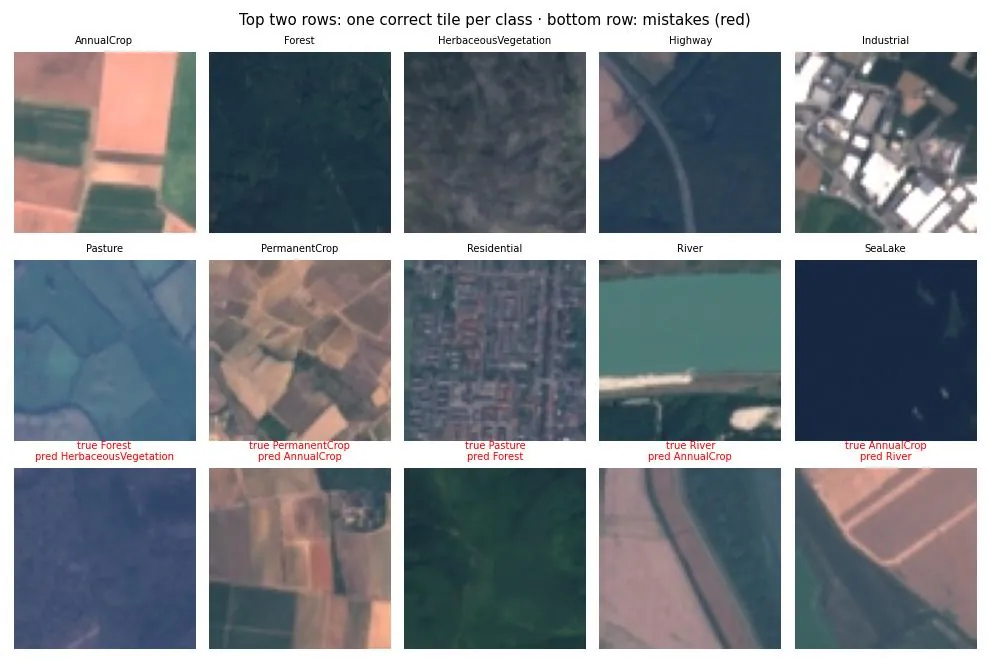
Top two rows: one correct tile per class. Bottom row: mistakes, mostly tiles that mix two land types (river and fields) or similar crop types.

Results

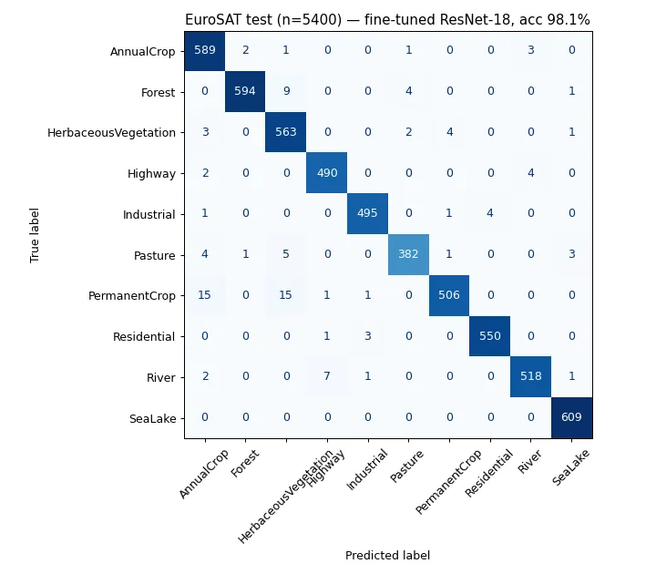
Standard EuroSAT RGB split, test set of 5,400 tiles.

Model	Training on EuroSAT	Test accuracy	Macro F1	CPU time / tile
ResNet-18 fine-tuned	16,200 tiles, 6 epochs	98.07 %	0.981	15.5 ms
CLIP ViT-B/32 zero-shot	none (text prompts only)	47.44 %	—	62.8 ms

Per-class F1 (fine-tuned): every class ≥ 0.964. Best: SeaLake 0.995, Residential 0.993; hardest: PermanentCrop 0.964, HerbaceousVegetation 0.966.

Why zero-shot fails here (and didn’t in project 17)

Class	CLIP zero-shot accuracy
Residential	93.9 %
Industrial	86.0 %
PermanentCrop	72.1 %
Highway	59.3 %
…	…
Forest	17.8 %
HerbaceousVegetation	0.7 %

CLIP learned from internet photos with captions. Buildings from above appear in such photos, so it recognizes Residential and Industrial; but a 64-pixel dark green square labeled “forest” looks nothing like the forests in its training data. In project 17 (COCO photos), zero-shot Grounding DINO beat a supervised YOLO. Zero-shot models are strong in-domain and weak out-of-domain; for specialized imagery (satellite, medical, industrial), a small fine-tuned model wins easily.

How it works

1. Data: tiles are decoded once into RAM (the whole set is tiny), then upsampled from 64 to 128 px so ImageNet filters see familiar scales.
2. Augmentation: horizontal/vertical flips and 90° rotations (satellite images have no “up”), plus brightness/contrast jitter.
3. Model: ResNet-18 (ImageNet weights, timm), new 10-class head, AdamW + one-cycle learning rate, label smoothing 0.05, 4 CPU threads (the performance cores, see project 19).
4. Zero-shot baseline: OpenCLIP ViT-B/32 (same model as project 16) with prompts "a satellite photo of {class}."; the class with the highest image-text similarity wins. evaluate.py reuses the model settings from ../16-text-to-image-search/clip_search.py, so that folder (and its faiss-cpu dependency) must be present.

Data

• EuroSAT RGB (Helber et al., 2019): 27,000 labeled Sentinel-2 tiles, 10 classes; Hugging Face mirror timm/eurosat-rgb (MIT) with the standard 16,200 / 5,400 / 5,400 split.
• Location: ../../cv-data/eurosat/ (not committed).

Run it

.venv\Scripts\activate            # shared environment, from the repo root
cd 12-satellite-land-cover
python train.py --epochs 6        # ~1 h on an idle CPU
python evaluate.py                # test accuracy, CLIP zero-shot, figures

What I learned / what didn’t work

• 98 % in 6 epochs. EuroSAT is close to solved; published ResNet results are in the same range, which makes it a good sanity check but not much of a challenge.
• The remaining errors are label ambiguity, not model failure: a 640 m × 640 m tile often contains two land types, and the label is the dominant one.
• Domain shift decides zero-shot quality (see above): the most useful finding of this project.
• Training time varied from 8 to 55 minutes per epoch because other jobs shared the CPU; on an idle CPU an epoch takes ~8–10 minutes.
• This is classification of whole tiles, not pixel-level segmentation. The original plan (LoveDA segmentation) needed 8 GB of data; EuroSAT fit the constraints.

Next steps

• Use all 13 Sentinel-2 spectral bands (EuroSAT MS): near-infrared separates vegetation types far better than RGB.
• Slide the classifier over a large satellite scene to produce a coarse land-cover map.
• Pixel-level segmentation on a larger dataset with a GPU.

Tech stack

Python · PyTorch · timm (ResNet-18) · OpenCLIP · scikit-learn · pyarrow